PyMOL: Mapping properties onto a structure - Electrostatic potential,
conservation, hydrophobicity/polarity, ...
There are at least two common possibilities to map properties
color-coded onto a cartoon, stick or surface representation: One can color
the atoms or residues directly via commands or one can use the spectrum
command, which colors a selection according to the
magnitude of values stored most commonly in the B-factor
column of a pdb file.
The spectrum command
Properties are typically mapped via the B-factor column onto a protein
structure, usually represented in cartoon mode or as molecular surface.
The most important command is:
spectrum
B, palette, selection, minimum, maximum
palette is one of the following options, describing the color
change from minimum to maximum:
| blue_white_red |
From cold (low values) to warm (high values), suitable
for mobility (root mean square fluctuations (rmsf) from MD
simulations, root mean square deviations (rmsd) from superpositions,
crystallographic temperature factors). |
| red_white_blue |
Inverse coloring, suitable for AlphaFold pLDDT values
(low values=low confidence=often disordered -> high values, high
confidence, well folded), charge or electrostatic potential (both:
red=negative, blue=positive). |
| rainbow or rainbow2 |
Similar blue to red via rainbow colors. |
| rainbow_rec or rainbow2_rev |
Inverse rainbow coloring. |
| color1 color 2 color3... |
In addition to the predefined palettes, you can also specify a
list of color names separated by blanks, which will generate a
gradient from color1 (minimum) to the last color of the list
(maximum). |
| more options here |
|
selection specifies the atoms that will be colored by the
B-factor, usually the Cα-atoms, as these define the
color of the fold or of the molecular surface. However, if you aim to
depict a property on individual atoms, such as the rmsd values of a ligand
in an MD simulation below, this is also possible.
minimum and maximum define the range of values to which
the color spectrum is extended. If you omit these values, the range
is determined automatically as the lowest and highest value present.
If these are extreme "outliers", it may be necessary to narrow the range
of spectrum color change by specifying the minimum and maximum values.
Examples
Click on the images to see the full resolution image.

|
Electrostatic
potential of the Y2R receptor. The electrostatic potential is
mapped onto the molecular surface of the Y2R receptor (PDB id 7yon).
This image was created with APBS plugin of PyMOL as
described here.
Note that the potential in the central membrane region does not
describe the physiological situation as the hydrophobic membrane was
not part of the calculation. Instead the potential was generated for
the receptor in water.
It is also possible to generate the electrostatic potential at the
molecular surface using a PyMOL function accessible via the object
buttons: OB: 7yon: A: generate, vacuum electrostatics, protein
contact potential. I assume that the calculation via APBS is
more sophisticated and allows for better control of the parameters
and the structure. |

|
Sequence conservation
of the pancreatic peptide. Conservation scores were
calculated with the ConSurf server. The pdb file was
downloaded and the scores were mapped onto the cartoon
representation via the following commands. High conservation is
indicated in pink, intermediate in white and low conservation in
cyan. The C-terminal residues binding into the Y2R pocket are
conserved. The very C-terminal tyrosine residue (drawn in red
here) was not correctly processed due to the "TYC" residue name.
It should have been renamed to TYR before the ConSurf analysis.
load 7yon_L_With_Conservation_Scores.pdb
hide all
show cartoon, chain L
spectrum b, hotpink white aquamarine, chain L, -1.5, 1.5
orient chain L
turn z, 90
util.performance(0)
draw 350,800 |

|
Sequence
conservation of the orthosteric ligand binding pocket of the Y2
receptor. Conservation scores were calculated with the ConSurf server. The pdb file was
downloaded and the scores were mapped onto the molecular
surface. High conservation is indicated in pink, intermediate in
white and low conservation in cyan. The commands are similar as in
the example above, with the exception that the surface is shown and
not the cartoon. The binding pocket is conserved
The cartoon representation is not so useful, as the buried
residues in the core of the protein always have higher
conservation scores than the residues on the protein surface,
for structural reasons. By mapping |

|
Sequence
conservation of the cytosolic interface of the Y2 receptor. |

|
Hydrophobicity of the molecular surface of the Y2
receptor. The hydrophobicity has been quantified according
to Eisenberg et al. J. Mol. Biol. 179:125-142
(1984). Using the pymol python script color_h.py,
which you also may download from here
and save it to a directory on your computer, a new command color_h
is defined, which colors the amino acids according to the Eisenberg
hydrophobicity scale. Using color_h increasing
hydrophobicity is indicated by red color. The script also defines
color_h2, which colors from green (polar) to grey
(hydrophobic). I would prefer to color hydrophobic regions yellow,
one would need to modify the color definitions on color_h.py to
achieve that. Syntax: color_h <selection>.
set bg_rgb,
white
fetch 7yon
remove not chain R
hide all
show surface, chain R
orient chain R
turn z, 90
run color_h.py
color_h |

|
Hydrophobicity
and charge of the molecular surface of the Y2 receptor.This
figure was generated using a python
script of Hagemans and van Belzen. Hydrophobic atoms are
colored yellow, positively charged groups blue and negatively
charged groups red. Look at the python script for further details or
changing the colors, which is easy for this script.
Syntax: color_yrb <selection>.
set bg_rgb,
white
fetch 7yon
remove not chain R
hide all
show surface, chain R
orient chain R
turn z, 90
run color_YRB.py
color_yrb |

|
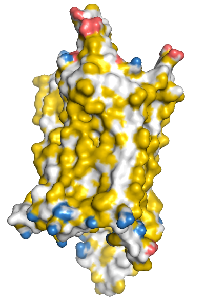
Mapping
charge, polarity and hydrophobicity onto the molecular surface.
In the following script, atoms are colored according to charge,
polarity and hydrophobicity and the corresponding molecular surface
is shown. As an alternative to the following pml script, one could
modify the color_YRB.py script to define a command for the coloring
steps.
fetch 7yon
remove not chain R or hydrogen
hide all
color white
# hydrophobic
color white, ele C+S
# polar
set_color c_polar, [1.0, 0.8, 0.0]
color paleyellow, name C+O+N
color c_polar, (resn SER and name OG) or (resn THR and name OG1)
color c_polar, (resn ASN and name CG+OD1+ND2) or (resn GLN and
name CD+OE1+NE2)
color c_polar, resn HIS and (sidechain and not name CB)
color c_polar, (resn TRP and name NE1) or (resn TYR and name OH)
# positive charge
color blue, (resn ARG and name NE+NH1+NH2+CZ) or (resn LYS and
name NZ)
# negative charge
color red, (resn ASP and name CG+OD1+OD2) or (resn GLU and name
CD+OE1+OE2)
show surface
|

|
Color
an AlphaFold model according to pLDDT values:
load
hsG4dimer_a13c4_unrelaxed_rank_1_model_2.pdb,
pdb1
set bg_rgb, white
dss
spectrum b, rainbow_rev
show cartoon
util.performance(0)
orient
turn x, 110
clip slab, 50 |
The following figure shows an example, where the atoms of a ligand
are color-coded by the root-mean-square fluctuations of a
molecular dynamics simulation. Blue color indicates low rmsf values,
i.e. low mobility, and red high rmsf values. In addition to the
color-coding, the rmsf values (in Å) are also listed next to the atoms.
The rmsf values were stored in the B-factor column and the spectrum
command was used to achieve the color-coding.


